Introduction to SimPy Classic
| Authors: | G A Vignaux and Klaus Muller |
|---|---|
| Date: | Feb 24, 2018 |
| Release: | 2.3.4 |
| Python-Version: | 2.7 and later |
Contents
Introduction
The active elements (or entities) of a SimPy model are objects of a class defined by the programmer (see Processes, section 3). Each entity has a standard method, a Process Execution Method (referred to by SimPy programmers as a PEM) which specifies its actions in detail. Each PEM runs in parallel with (and may interact with) the PEMs of other entities.
The activity of an entity may be delayed for fixed or random times, queued at resource facilities, and may be interrupted by or interact in different ways with other entities and components. For example in a gas station model, automobile entities (objects of an Automobile Class) may have to wait at the gas station for a pump to become available. On obtaining a pump it takes time to fill the tank. The pump is then released for the next automobile in the queue if there is one.
SimPy has three kinds of resource facilities (Resources, Levels, and Stores). Each type models a congestion point where entities queue while waiting to acquire or, in some cases, to deposit a resource.SimPy automatically handles the queueing.
- Resources have one or more identical resource units, each of which can be held by entities. Extending the example above, the gas station might be modelled as a Resource with its pumps as resource units. When a car requests a pump the gas station resource automatically queues it until a pump becomes available (perhaps immediately). The car holds the pump until it finishes refuelling and then releases it for use by the next car.
Levels(not treated here) model the supply and consumption of a homogeneous undifferentiated “material”. The Level holds an amount that is fully described by a non-negative number which can be increased or decreased by entities. For example, a gas station stores gas in large storage tanks. The tanks can be filled by tankers and emptied by cars refuelling. In contrast to the operation of a Resource, a car need not return the gas to the gas station.
Stores(not treated here) model the production and consumption of distinguishable items. A Store holds a list of items. Entities can insert or remove items from the list and these can be of any type. They can even be SimPy process objects. For example, the gas station holds spares of different types. A car might request a set of spares from the Store. The store is replenished by deliveries from a warehouse.
SimPy also supplies Monitors and Tallys to record simulation events. Monitors are used to compile summary statistics such as waiting times and queue lengths. These statistics includes simple averages and variances, time-weighted averages, or histograms. In particular, data can be gathered on the queues associated with Resources, Levels and Stores. For example we may collect data on the average number of cars waiting at the gas station and the distribution of their waiting times. Monitors preserve complete time-series records that may later be used for more advanced post-simulation analyses. A simpler version of a Monitor is a Tally which provides most of the statistical facilities but does not retain a complete time-series record. See the SimPy Manual for details on the Tally.
Simulation with SimPy
To use the SimPy simulation system in your Python program you must import its
Simulation module using:
from SimPy.Simulation import *
We recommend that new users instead import SimPy.SimulationTrace,
which works the same but also automatically produces a timed listing of
events as the model executes. (An example of such a trace is shown in
The Resource Example with Tracing):
from SimPy.SimulationTrace import *
Discrete-event simulation programs automatically maintain the current
simulation time in a software clock. This cannot be directly changed
by the user. In SimPy the current clock value is returned by the
now() function and you can access this or print it out. At the
start of the simulation it is set to 0.0. While the simulation
program runs, simulation time steps forward from one event to the
next. An event occurs whenever the state of the simulated system
changes such as when a car arrives or departs from the gas station.
The initialize statement initialises global simulation variables and
sets the software clock to 0.0. It must appear in your program before
any SimPy process objects are activated.
initialize()
This is followed by SimPy statements creating and activating entities (that is, SimPy process objects). Activation of entities adds events to the simulation event schedule. Execution of the simulation itself starts with the following statement:
simulate(until=endtime)
The simulation then starts, and SimPy seeks and executes the first event in the schedule. Having executed that event, the simulation seeks and executes the next event, and so on.
Typically a simulation terminates when there are no more events to execute or when the endtime is reached but it can be stopped at any time by the command:
stopSimulation( )
After the simulation stops, further statements can be executed.
now() will retain the time of stopping and data held in Monitors
will be available for display or further analysis.
The following fragment shows only the main block in a simulation
program to illustrate the general structure. A complete Example
Program is shown later. Here Car is a Process class with a
go as its PEM (described later) and c is made an entity of
that class, that is, a particular car. Activating c has the effect
of scheduling at least one event by starting c’s PEM. The
simulate(until=1000.0) statement starts the simulation
itself. This immediately jumps to the first scheduled event. It will
continue executing events until it runs out of events to execute or
the simulation time reaches 1000.0. When the simulation stops the
Report function is called to display the results:
1 2 3 4 5 6 7 8 9 10 11 12 13 14 15 | class Car(Process):
def go(self):
# PEM for a Car
...
def Report():
# print results when finished
...
initialize()
c = Car(name="Car23")
activate(c, c.go(), at=0.0)
simulate(until=1000.0)
Report()
|
In addition to SimPy.Simulation there are three alternative
simulation libraries with the same simulation capabilities but with
special facilities. Beside SimPy.SimulationTrace, already
mentioned, there are SimPy.SimulationRT for real time
synchronisation and SimPy.SimulationStep for event-stepping through
a simulation. See the SimPy Manual for more information.
Processes
SimPy’s active objects (entities) are process objects – instances of a class written by the user that inherits from SimPy’s Process class.
For example, if we are simulating a gas station we might model each
car as an object of the class Car. A car arrives at the gas
station (modelled as a Resource with pumps). It requests a pump
and may need to wait for it. Then it fills its tank and when it has
finished it releases the pump. It might also buy an item from the
station store. The Car class specifies the logic of these actions
in its Process Execution Method (PEM). The simulation creates a number
of cars as it runs and their evolutions are directed by their Car
class’s PEM.
Defining a process
Each Process class inherits from SimPy’s Process class. For example
the header of the definition of a Car Process class would
be:
class Car(Process):
At least one Process Execution Method (PEM) must be defined in each
Process class (though an entity can have only one PEM active). A PEM
may have arguments in addition to the required self argument
needed by all Python class methods. Naturally, other methods and, in
particular, an __init__, may be defined.
A Process Execution Method (PEM)defines the actions that are performed by its process objects. Each PEM must contain at least one of the special ``yield`` statements, described later. This makes the PEM a Python generator function so that it has resumable execution – it can be restarted again after the yield statement without losing its current state. A PEM may have any name of your choice. For example it may be calledexecute( )orrun( ). However, if a PEM is calledACTIONS, SimPy recognises this as a PEM. This can simplify thestartmethod as explained below.The
yieldstatements are simulation commands which affect an ongoing life cycle of Process objects. These statements control the execution and synchronisation of multiple processes. They can delay a process, put it to sleep, request a shared resource or provide a resource. They can add new events to the simulation event schedule, cancel existing ones, or cause processes to wait for a change in the simulated system’s state.For example, here is a Process Execution Method,
go(self), for the simpleCarclass that does no more than delay for a time. As soon as it is activated it prints out the current time, the car object’s name and the wordStarting. After a simulated delay of 100.0 time units (in theyield hold, ...statement) it announces that this car has “Arrived”:def go(self): print("%s %s %s" % (now(), self.name, 'Starting')) yield hold, self, 100.0 print("%s %s %s" % (now(), self.name, 'Arrived'))
A process object’s PEM starts execution when the object is activated, provided the
simulate(until=endtime)statement has been executed.__init__(self, …), where … indicates other arguments. This method is optional but is useful to initialise the process object, setting values for its attributes. As for any sub-class in Python, the first line of this method must call the
Processclass’s__init__( )method in the form:Process.__init__(self)You can then use additional commands to initialise attributes of the Process class’s objects. You can also override the standard
nameattribute of the object.If present, the
__init__( )method is always called whenever you create a new process object. If you do not wish to provide for any attributes other than aname, the__init__method may be dispensed with. An example of an__init__( )method is shown in the Example Program.
Creating a process object
An entity (process object) is created in the usual Python manner by
calling the Class. Process classes have a single attribute, name
which can be specified even if no __init__ method is defined. name
defaults to 'a_process' unless the user specified a different one.
For example to create a new Car object with a name Car23:
c = Car(name="Car23")
Starting SimPy Process Objects
An entity (process object) is “passive” when first created, i.e., it
has no events scheduled for it. It must be activated to start its
Process Execution Method. To do this you can use either the
activate function or the start method of the Process.
activate
Activating an entity by using the SimPy activate function:
activate(p, p.pemname([args])[,{at=t|delay=period}])activates process object p, provides its Process Execution Method p.pemname( ) with the arguments args and possibly assigns values to the other optional parameters. You must choose one (or neither) of
at=t anddelay=period. The default is to activate at the current time (at=now( )) and with no delay (delay=0).For example: to activate an entity,
custat time 10.0 using its PEM calledlifetime:cust = Customer() activate(cust, cust.lifetime(), at=10.0)
start
An alternative to the activate() function is the start method
of Process objects:
p.
start(p.pemname([args])[,{at=t|delay=period}])Here p is a Process object. Its PEM, pemname, can have any identifier (such as
run,lifecycle, etc) and any arguments args.For example, to activate the process object
custusing the PEM with identifierlifetimeat time 10.0 we would use:cust.start(cust.lifetime(), at=10.0)
The standard PEM name, ACTIONS
The identifier ACTIONS is recognised by SimPy as a PEM name and
can be used (or implied) in the start method.
p.
start([p.ACTIONS()][,{at=t|delay=period}])ACTIONScannot have parameters. The call p.ACTIONS()is optional but may make your code clearer.For example, to activate the Process object
custwith a PEM calledACTIONSat time 10.0, the following are equivalent (and the second version more convenient):cust.start(cust.ACTIONS(), at=10.0) cust.start(at=10.0)
A reminder: Even activated process objects will not actually start
operating until the simulate() statement is executed.
Elapsing time in a Process
A PEM uses the yield hold command to temporarily delay a process
object’s operations. This might represent a service time for the
entity. (Waiting is handled automatically by the resource facilities
and is not modelled by yield hold)
yield hold
yield hold, self, tCauses the entity to delay t time units. After the delay, it continues with the next statement in its PEM. During the
holdthe entity’s operations are suspended.
Paradoxically, in the model world, the entity is considered to be busy during this simulated time. For example, it might be involved in filling up with gas or driving. In this state it can be interrupted by other entities.
More about Processes
An entity (Process object) can be “put to sleep” or passivated using
yield passivate, self
(and it can be reactivated by another entity
using reactivate), or permanently removed from the future event
queue by the command self.cancel(). Active entities can be
interrupted by other entities. Examine the full SimPy Manual for
details.
A SimPy Program
This is a complete SimPy script. We define a Car class with a PEM
called go( ). We also (for interest) define an __init__( )
method to provide individual cars with an identification name and
engine size, cc. The cc attribute is not used in this very
simple example.
Two cars, p1 and p2 are created. p1 and p2 are
activated to start at simulation times 0.6 and 0.0, respectively. Note
that these will not start in the order they appear in the program
listing. p2 actually starts first in the simulation. Nothing
happens until the simulate(until=200) statement at which point the
event scheduler starts operating by finding the first event to
execute. When both cars have finished (at time 6.0+100.0=106.0)
there will be no more events so the simulation will stop:
from SimPy.Simulation import Process, activate, hold, initialize, now, simulate


class Car(Process):
    def __init__(self, name, cc):
        Process.__init__(self, name=name)
        self.cc = cc

    def go(self):
        print('%s %s %s' % (now(), self.name, 'Starting'))
        yield hold, self, 100.0
        print('%s %s %s' % (now(), self.name, 'Arrived'))


initialize()
c1 = Car('Car1', 2000)                # a new car
activate(c1, c1.go(), at=6.0)    # activate at time 6.0
c2 = Car('Car2', 1600)                # another new car
activate(c2, c2.go())                # activate at time 0
simulate(until=200)
print('Current time is %s' % now())    # will print 106.0
Running this program gives the following output:
0 Car2 Starting
6.0 Car1 Starting
100.0 Car2 Arrived
106.0 Car1 Arrived
Current time is 106.0
If, instead one chose to import SimPy.SimulateTrace at the start
of the program one would obtain the following output. (The meaning of
the phrase prior : False in the first two lines is described in
the full SimPy Manual. prior is an advanced technique for fine control
of PEM priorities but seldom affects simulated operations and so
normally can be ignored/)
0 activate <Car1> at time: 6.0 prior: False
0 activate <Car2> at time: 0 prior: False
0 Car2 Starting
0 hold <Car2> delay: 100.0
6.0 Car1 Starting
6.0 hold <Car1> delay: 100.0
100.0 Car2 Arrived
100.0 <Car2> terminated
106.0 Car1 Arrived
106.0 <Car1> terminated
Current time is 106.0
Resources
The three resource facilities provided by SimPy are Resources,
Levels and Stores. Each models a congestion point where process
objects may have to queue up to access resources. This section
describes the Resource type of resource facility. Levels and
Stores are not treated in this introduction.
An example of queueing for a Resource might be a manufacturing plant
in which a Task (modelled as an entity or Process object) needs
work done by a Machine (modelled as a Resource object). If all
of the Machines are currently being used, the Task must wait
until one becomes free. A SimPy Resource can have a number of
identical units, such as a number of identical machine
units. An entity obtains a unit of the Resource by requesting it
and, when it is finished, releasing it. A Resource maintains a
list (the waitQ) of entities that have requested but not yet
received one of the Resource’s units, and another list (the
activeQ) of entities that are currently using a unit. SimPy
creates and updates these queues itself – the user can read their
values, but should not change them.
Defining a Resource object
A Resource object, r, is established by the following statement:
r = Resource(capacity=1,
             name='a_resource',
             unitName='units',
             monitored=False)
where
capacity(positive integer) specifies the total number of identical units in Resource objectr.
name(string) the name for this Resource object (e.g.,'gasStation').
unitName(string) the name for a unit of the resource (e.g.,'pump').
monitored(FalseorTrue) If set toTrue, then information is gathered on the sizes ofr’swaitQandactiveQ, otherwise not.
For example, in the model of a 2-pump gas-station we might define:
gasstation = Resource(capacity=2, name='gasStation', unitName='pump')
Each Resource object, r, has the following additional attributes:
r.n, the number of units that are currently free.
r.waitQ, a queue (list) of processes that have requested but not yet received a unit ofr, solen(r.waitQ)is the number of process objects currently waiting.
r.activeQ, a queue (list) of process objects currently using one of the Resource’s units, solen(r.activeQ)is the number of units that are currently in use.
r.waitMon, the record (made by aMonitorwhenevermonitored == True) of the activity inr.waitQ. So, for example,r.waitMon.timeaverage()is the average number of processes inr.waitQ. See Data Summaries for an example.
r.actMon, the record (made by aMonitorwhenevermonitored==True) of the activity inr.activeQ.
Requesting and releasing a unit of a Resource
A process can request and later release a unit of the Resource object,
r, by using the following yield commands in a Process Execution
Method:
yield request
yield request,self,r
Requests a unit of Resource r
If a Resource unit is free when the request is made, the requesting
entity takes it and moves on to the next statement in its PEM. It is
added to the Resource’s activeQ.
If no Resource unit is available when the request is made, the
requesting entity is appended to the Resource’s waitQ and
suspended. The next time a unit becomes available the first entity in
the r.waitQ takes it and continues its execution.
For example, a Car might request a pump:
yield request, self, gasstation
(It is actually requesting a unit of the gasstation, i.e. a
pump.) An entity holds a resource unit until it releases it.
Entities can use a priority system for queueing. They can also preempt
(that is, interrupt) others already in the system. They can also
renege from the waitQ (that is, abandon the queue if it takes
too long). This is achieved by an extension to the yield request
command. See the main SimPy Manual.
yield release
yield release, self, r
Releases the unit of r.
The entity is removed from r.activeQ and continues with its next
statement. If, when the unit of r is released, another entity is
waiting (in waitQ) it will take the unit, leave the waitQ and
move into the activeQ and go one with its PEM.
For example the Car might release the pump unit of the
gasstation:
yield release, self, gasstation
Resource Example
In this complete script, the gasstation Resource object is given
two resource units (capacity=2). Four cars arrive at the times
specified in the program (not in the order they are listed). They all
request a pump and use it for 100 time units:
1 2 3 4 5 6 7 8 9 10 11 12 13 14 15 16 17 18 19 20 21 22 23 24 25 26 27 28 29 30 | from SimPy.Simulation import (Process, Resource, activate, initialize, hold,
now, release, request, simulate)
class Car(Process):
def __init__(self, name, cc):
Process.__init__(self, name=name)
self.cc = cc
def go(self):
print('%s %s %s' % (now(), self.name, 'Starting'))
yield request, self, gasstation
print('%s %s %s' % (now(), self.name, 'Got a pump'))
yield hold, self, 100.0
yield release, self, gasstation
print('%s %s %s' % (now(), self.name, 'Leaving'))
gasstation = Resource(capacity=2, name='gasStation', unitName='pump')
initialize()
c1 = Car('Car1', 2000)
c2 = Car('Car2', 1600)
c3 = Car('Car3', 3000)
c4 = Car('Car4', 1600)
activate(c1, c1.go(), at=4.0) # activate at time 4.0
activate(c2, c2.go()) # activate at time 0.0
activate(c3, c3.go(), at=3.0) # activate at time 3.0
activate(c4, c4.go(), at=3.0) # activate at time 2.0
simulate(until=300)
print('Current time is %s' % now())
|
This program results in the following output:
0 Car2 Starting
0 Car2 Got a pump
3.0 Car3 Starting
3.0 Car3 Got a pump
3.0 Car4 Starting
4.0 Car1 Starting
100.0 Car2 Leaving
100.0 Car4 Got a pump
103.0 Car3 Leaving
103.0 Car1 Got a pump
200.0 Car4 Leaving
203.0 Car1 Leaving
Current time is 203.0
And, if we use SimPy.SimulationTrace to get an automatic trace we
get the result shown in Appendix The Resource Example with Tracing.
(It is rather long to be inserted here).
Random Number Generation
Simulations usually need random numbers. By design, SimPy does not provide its own random number generators, so users need to import them from some other source. Perhaps the most convenient is the standard Python random module. It can generate random variates from the following continuous distributions: uniform, beta, exponential, gamma, normal, log-normal, Weibull, and vonMises. It can also generate random variates from some discrete distributions. Consult the module’s documentation for details. Excellent brief descriptions of these distributions, and many others, can be found in the Wikipedia.
Python’s random module can be used in two ways: you can import the
methods directly or you can import the Random class and make your
own random objects. In the second method, each object gives a
different random number sequence, thus providing multiple random
streams as in some other simulation languages such as Simscript and
ModSim.
Here the first method is illustrated. A single pseudo-random sequence
is used for all calls. You import the methods you need from the
random module. For example:
from random import seed, random, expovariate, normalvariate
In simulation it is good practice to set the initial seed for the
pseudo-random sequence at the start of each run. You then have good
control over the random numbers used. Replications and comparisons are
easier and, together with variance reduction techniques, can provide
more accurate estimates. In the following code snippet we set the
initial seed to 333555. X and Y are pseudo-random
variates from the two distributions. Both distributions have the same
mean:
1 2 3 4 5 | from random import seed, expovariate, normalvariate
seed(333555)
X = expovariate(0.1)
Y = normalvariate(10.0, 1.0)
|
Monitors and Recording Simulation Results
A Monitor enables us to observe a particular variable of interest and to hold a time series of its values. It can return a simple data summary either during or at the completion of a simulation run.
For example we might use one Monitor to record the waiting time for each of a series of customers and another to record the total number of customers in the shop. In a discrete-event system the number of customers changes only at arrival or departure events and it is at those events that the number in the shop must be observed. A Monitor provides simple statistics useful either alone or as the start of a more sophisticated statistical analysis.
When Resources are defined, a Monitor can be set up to automatically observe the lengths of each of their queues.
The simpler version, the Tally, is not covered in this document. See the SimPy Manual for more details.
Defining Monitors
The Monitor class preserves a complete time-series of the observed
data values, y, and their associated times, t. The data are held
in a list of two-item sub-lists, [t,y]. Monitors calculate data
summaries using this time-series when your program requests them. In
long simulations their memory demands may be a disadvantage
To define a new Monitor object:
m = Monitor(name='a_Monitor')where
nameis a descriptive name for the Monitor object. The descriptive name is used when the data is graphed or tabulated.
For example, to record the waiting times of cars in the gas station we might use a Monitor:
waittimes = Monitor(name='Waiting times')
Observing data
Monitors use their observe method to record data. Here and in the
next section, m is a Monitor object:
m.observe(y [,t])records the current value of the variable,
yand time t (or the current time,now(), if t is missing). A Monitor retains the two values as a sub-list[t,y].
For example, using the Monitor in the previous example, we might
record the waiting times of the cars as shown in the following
fragment of the PEM of a Car:
1 2 3 4 5 | startwaiting = now() # start wait
yield request, self, gasstation
waitingtime = now() - startwaiting # time spent waiting
waittimes.observe(waitingtime)
|
The first three lines measure the waiting time (from the time of the
request to the time the pump is obtained). The last records the
waiting time in the waittimes Monitor.
The data recording can be reset to start at any time in the
simulation:
m.reset([t])resets the observations. The recorded data is re-initialised, and the observation starting time is set to t, or to the current simulation time,
now( ), if t is missing.
Data summaries
The following simple data summaries are available from Monitors at any time during or after the simulation run:
m[i]holds thei-th observation as a two-item list, [ti, yi]
m.yseries( )is a list of the recorded data values, yi
m.tseries( )is a list of the recorded times, ti
m.count( ), the current number of observations. (This is the same aslen(r)).
m.total( ), the sum of theyvalues
m.mean( ), the simple numerical average of the observed y values, ignoring the times at which they were made. This ism.total( )/m.count( ).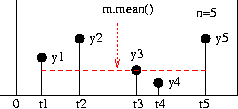
m.meanis the simple average of the y values observed.
m.var( )the sample variance of the observations, ignoring the times at which they were made. If an unbiased estimate of the population variance is desired, the sample variance should be multiplied by n/(n-1), where n = m.count( ). In either case the standard deviation is, of course, the square-root of the variance
m.timeAverage([t])the time-weighted average ofy, calculated from time 0 (or the last timem.reset([t])was called) to time t (or to the current simulation time,now(), if t is missing).This is intended to measure the average of a quantity that always exists, such as the length of a queue or the amount in a Level [1]. In discrete-event simulation such quantity changes are always instantaneous jumps occurring at events. The recorded times and new levels are sufficient information to calculate the average over time. The graph shown in the figure below illustrates the calculation. The total area under the line is calculated and divided by the total time of observation. For accurate time-average results y must be piecewise constant like this and observed just after each change in its value. That is, the y value observed must be the new value after the state change.
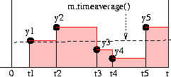
m.timeAverage([t])is the time-weighted average of the observedyvalues. Eachyvalue is weighted by the time for which it exists. The average is the area under the above curve divided by the total time, t.[1] timeAverageis not intended to measure instantaneous values such as a service time or a waiting time.m.mean()is used for that.
m.timeVariance([t])the time-weighted variance of theyvalues calculated from time 0 (or the last timem.reset([t])was called) to time t (or to the current simulation time,now(), if t is missing).
m.__str__( )is a string that briefly describes the current state of the monitor. This can be used in a print statement.
Monitoring Resource Queues
If a Resource, m, (and similarly for a Level or a Store) is
defined with monitored=True, SimPy automatically records the
lengths of its associated queues (i.e. waitQ and activeQ for
Resources, and the analogous queues for Levels and Stores). These
records are kept in Monitors m.waitMon for the waitQ and
m.actMon for the activeQ (and analogously for the other
resource types). This solves a problem, particularly for the waitQ
which cannot easily be recorded externally to the resource.
Complete time series for queue lengths are maintained and can be used for advanced post-simulation statistical analyses and to display summary statistics.
More on Monitors
When a Monitor is defined it is automatically entered into a global
list allMonitors. Each Monitor also has a descriptive label for
its variable values, y, and their corresponding times, t, that can
be used when the data are plotted. The function startCollection()
can be called to initialise all the Monitors in allMonitors at a
certain simulation time. This is helpful when a simulation needs a
‘warmup’ period to achieve steady state before measurements are
started. A Monitor can also generate a Histogram of the data
(The SimPy Tally is an alternative to Monitor that does essentially
the same job but uses less storage space at some cost of speed and
flexibility. See the SimPy Manual for more information on these options.)
Appendices
The Resource Example with Tracing
This is the trace produced in the Resource example when
SimPy.SimulationTrace is imported at the head of the program. The
relevance of the phrases `prior: False` and `priority:
default` refer to advanced but seldom-needed methods for
fine-grained control of event timing, as explained in the SimPy Manual. The
trace contains the results of all the print output specifically
called for by the user’s program (for example, line 5) but adds a line
for every event executed. (The request at time 3.0, for
example, lists the contents of the waitQ and the activeQ for
the gasstation.)
1 2 3 4 5 6 7 8 9 10 11 12 13 14 15 16 17 18 19 20 21 22 23 24 25 26 27 28 29 30 31 32 33 34 35 36 37 38 39 40 41 42 43 44 45 46 47 48 49 50 51 | 0 activate <Car1> at time: 4.0 prior: False
0 activate <Car2> at time: 0 prior: False
0 activate <Car3> at time: 3.0 prior: False
0 activate <Car4> at time: 3.0 prior: False
0 Car2 Starting
0 request <Car2> <gasStation> priority: default
. . .waitQ: []
. . .activeQ: ['Car2']
0 Car2 Got a pump
0 hold <Car2> delay: 100.0
3.0 Car3 Starting
3.0 request <Car3> <gasStation> priority: default
. . .waitQ: []
. . .activeQ: ['Car2', 'Car3']
3.0 Car3 Got a pump
3.0 hold <Car3> delay: 100.0
3.0 Car4 Starting
3.0 request <Car4> <gasStation> priority: default
. . .waitQ: ['Car4']
. . .activeQ: ['Car2', 'Car3']
4.0 Car1 Starting
4.0 request <Car1> <gasStation> priority: default
. . .waitQ: ['Car4', 'Car1']
. . .activeQ: ['Car2', 'Car3']
100.0 reactivate <Car4> time: 100.0 prior: 1
100.0 release <Car2> <gasStation>
. . .waitQ: ['Car1']
. . .activeQ: ['Car3', 'Car4']
100.0 Car2 Leaving
100.0 <Car2> terminated
100.0 Car4 Got a pump
100.0 hold <Car4> delay: 100.0
103.0 reactivate <Car1> time: 103.0 prior: 1
103.0 release <Car3> <gasStation>
. . .waitQ: []
. . .activeQ: ['Car4', 'Car1']
103.0 Car3 Leaving
103.0 <Car3> terminated
103.0 Car1 Got a pump
103.0 hold <Car1> delay: 100.0
200.0 release <Car4> <gasStation>
. . .waitQ: []
. . .activeQ: ['Car1']
200.0 Car4 Leaving
200.0 <Car4> terminated
203.0 release <Car1> <gasStation>
. . .waitQ: []
. . .activeQ: []
203.0 Car1 Leaving
203.0 <Car1> terminated
Current time is 203.0
|